Scalable Training and Rendering of 3D Gaussians for Large-Scale Scientific Data
Andres Sewell, Mengjiao Han, Qi Wu, and Steve Petruzza
ACM Computer Graphics and Interactive Techniques, 2026
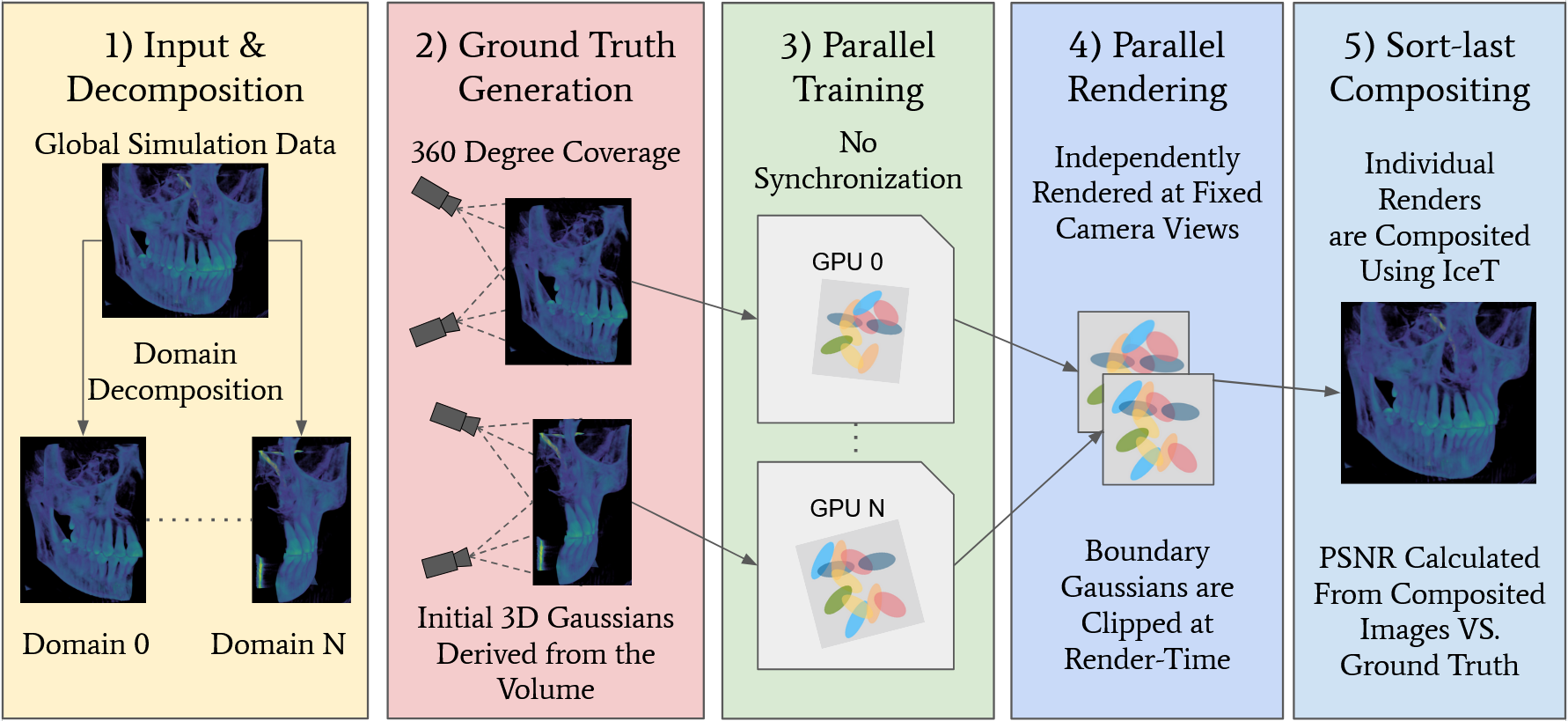
This framework maps the native spatial decomposition of an HPC simulation directly onto independent 3D Gaussian optimization tasks. Training requires no model synchronization or device-to-device exchange; boundary continuity is recovered with ghost cells and fragment-level clipping, and the local renders are combined only during sort-last compositing.
Abstract
The application of machine learning techniques to 3D Gaussian Splatting (3DGS) has enabled high-fidelity interactive rendering of complex 3D scenes on modest compute resources, offering significant potential for scientific visualization. However, reconstructing large scientific volumes at high fidelity exceeds the memory capacity of individual GPUs. Existing distributed 3DGS frameworks target urban scenes and depend on global scene analysis or frequent all-to-all communication, limiting their scalability on HPC clusters.
We present a distributed 3DGS training and rendering framework designed for large-scale scientific volume data. The method uses the native domain decomposition of HPC simulations and treats each spatial partition as an independent optimization task. It further exploits temporal coherence to accelerate later simulation timesteps. Experiments demonstrate near-ideal weak scaling by eliminating synchronization overhead. The study also characterizes the trade-off between standard 3DGS optimization, which provides higher fidelity with growing primitive counts, and MCMC optimization, which bounds model size at a dataset-dependent quality cost.
Why Scientific Data Is Different
Distributed simulations already partition their data across ranks, know the world-space bounds of each partition, and commonly maintain halo regions for numerical methods. A scientific visualization pipeline can use that structure directly. Photogrammetry-oriented distributed 3DGS systems instead maintain a globally consistent scene through parameter exchange or centralized image and gradient aggregation.
| System | Optimization unit | Training communication | Observed scaling behavior |
|---|---|---|---|
| Grendel-GS | Globally coordinated model | NCCL all-to-all or all-reduce | Communication bottleneck beyond 64 GPUs |
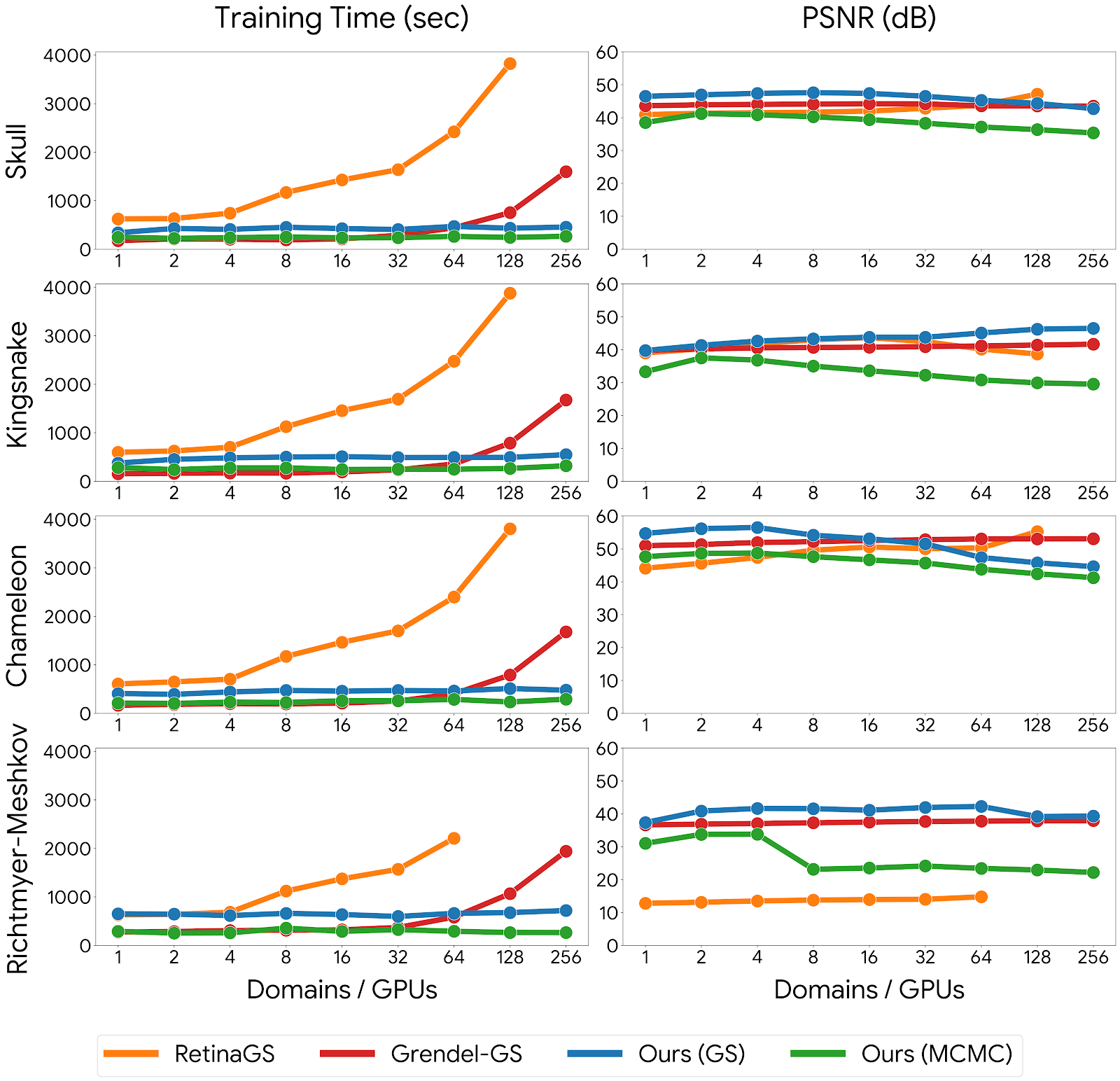
| RetinaGS | Partitioned workers with a central manager | Image collection, compositing, and gradient redistribution | More than 3,800 seconds at 128 GPUs; 256-GPU runs omitted |
| This work | Independent model per simulation subdomain | None during training | Near-constant time through 256 GPUs |
System Design
Use native simulation partitions or transfer-function-weighted recursive bisection, plus one ghost-cell layer.
Sample initial Gaussians from voxels and render 306 deterministic training views for each domain.
Assign one subdomain to each GPU and optimize using only local data, images, and gradients.
Clip fragments to primary domain bounds and use IceT to composite local color and depth buffers.
Domain decomposition and initialization
The evaluation harness recursively bisects the volume along its longest physical axis, selecting split planes that balance accumulated transfer-function opacity rather than raw voxel count. Highly visible structures receive smaller spatial partitions, while mostly transparent regions receive larger ones. Each partition receives the same initial primitive budget.
One ghost-cell layer extends each partition across shared boundaries. This supplies both neighboring optimizers with the same underlying scalar field around the split plane. Production simulation codes already maintain such halo data, so the method does not require a new category of boundary storage. Each subdomain initializes from 250,000 randomly sampled voxel centers and uses 300 Fibonacci-sphere views plus six axis-aligned views for deterministic 360-degree coverage.
Communication-free optimization
Every GPU trains a self-contained local 3DGS model from its own volume slice, ground-truth images, and gradients. No parameter consensus, gradient reduction, or global loss is computed during optimization. The wall-clock time is therefore governed by the slowest local partition rather than by a growing collective-communication cost.
Seamless Domain Boundaries
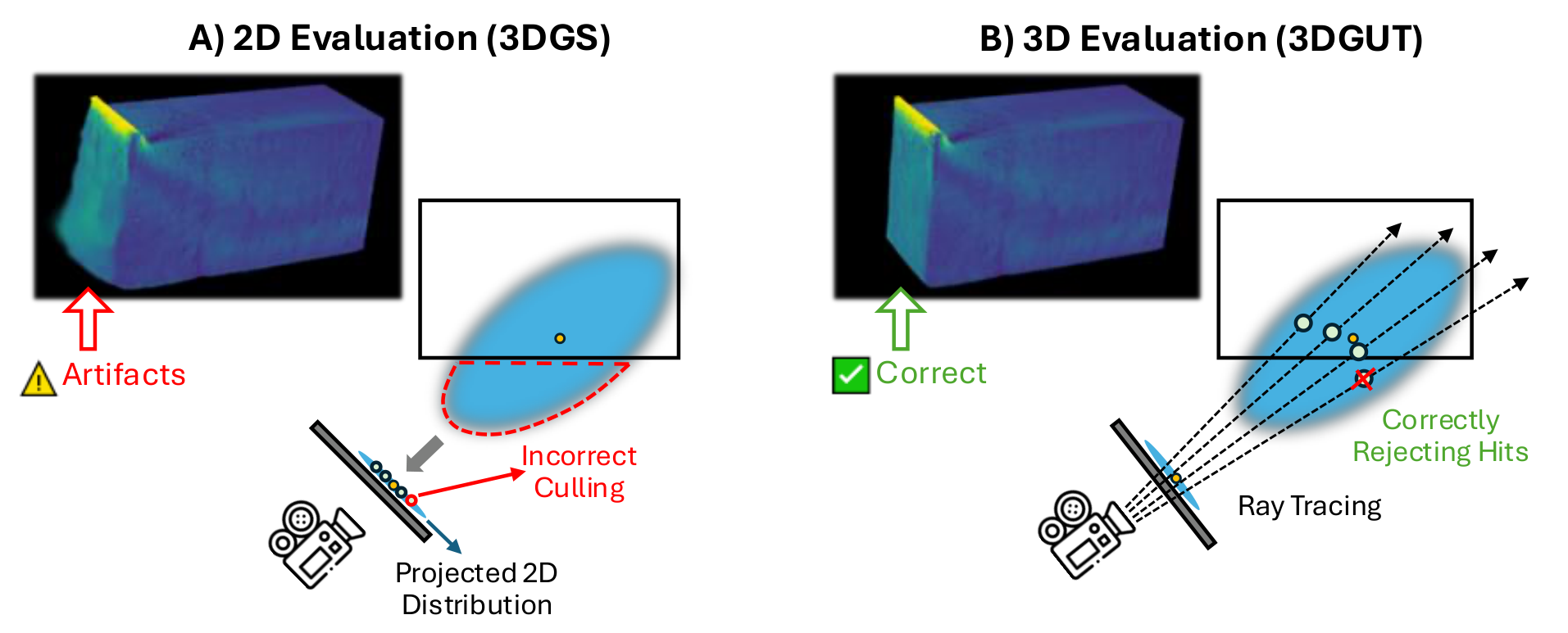
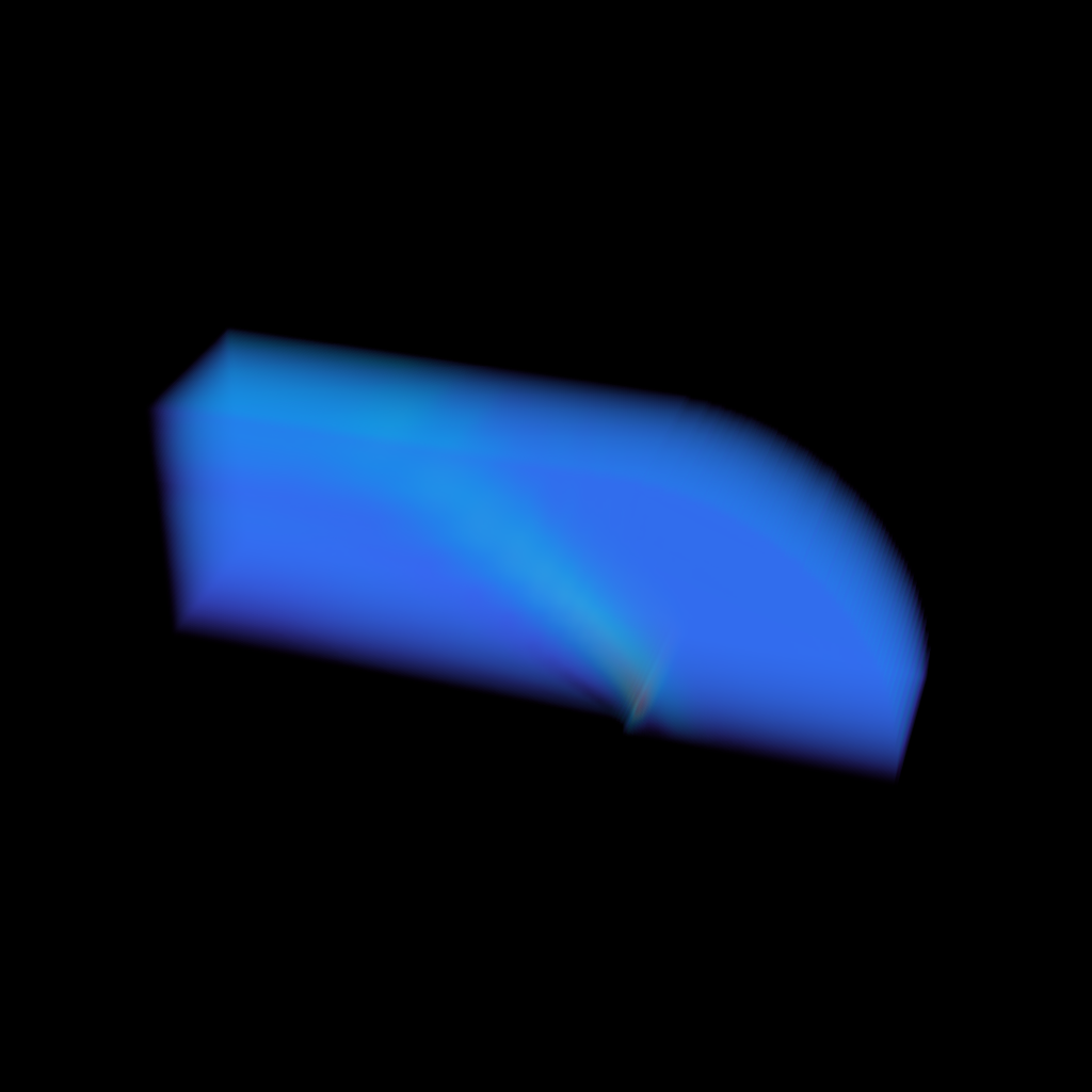
Independent Gaussians naturally extend beyond their assigned partitions. Discarding a Gaussian by its center creates gaps, while rendering its full projected footprint produces overlapping seams. The method instead modifies the 3DGUT rasterizer to intersect each ray with the primary domain’s axis-aligned bounding box. Contributions outside the box are rejected per fragment, retaining the useful portion of a Gaussian that straddles the boundary.
 Ground truth
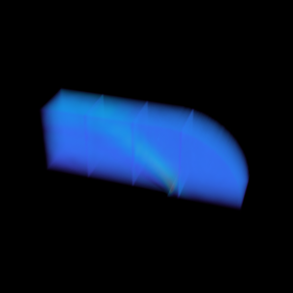 No culling
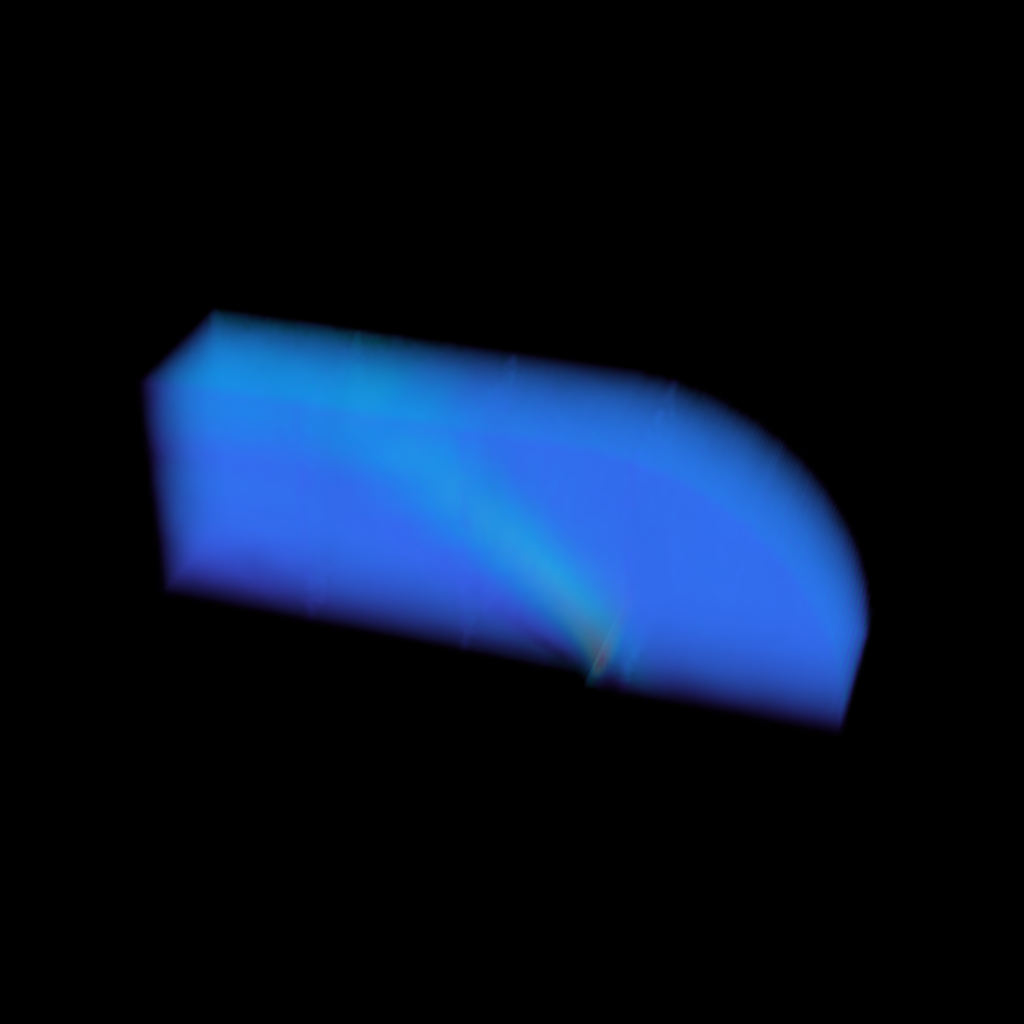 Center culling
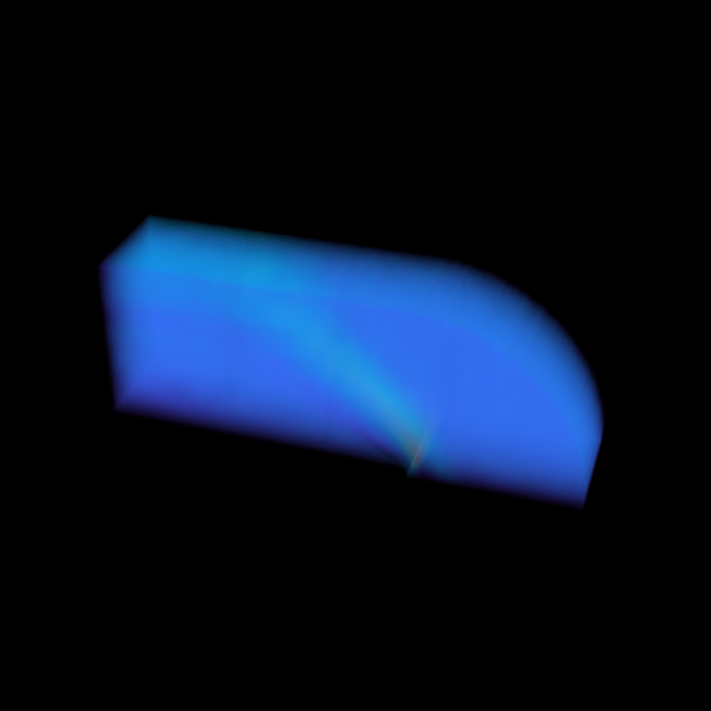 Fragment clipping
Evaluation at Scale
The communication-free GS pipeline maintains roughly constant per-dataset training time after the initial transition from one to multiple domains. Grendel-GS is faster at small GPU counts but its communication cost rises sharply after 64 GPUs. RetinaGS exceeds 3,800 seconds at 128 GPUs across completed runs, approximately 7.5-9x slower than this method, while its RMI reconstruction does not converge.
Standard GS or Bounded MCMC?
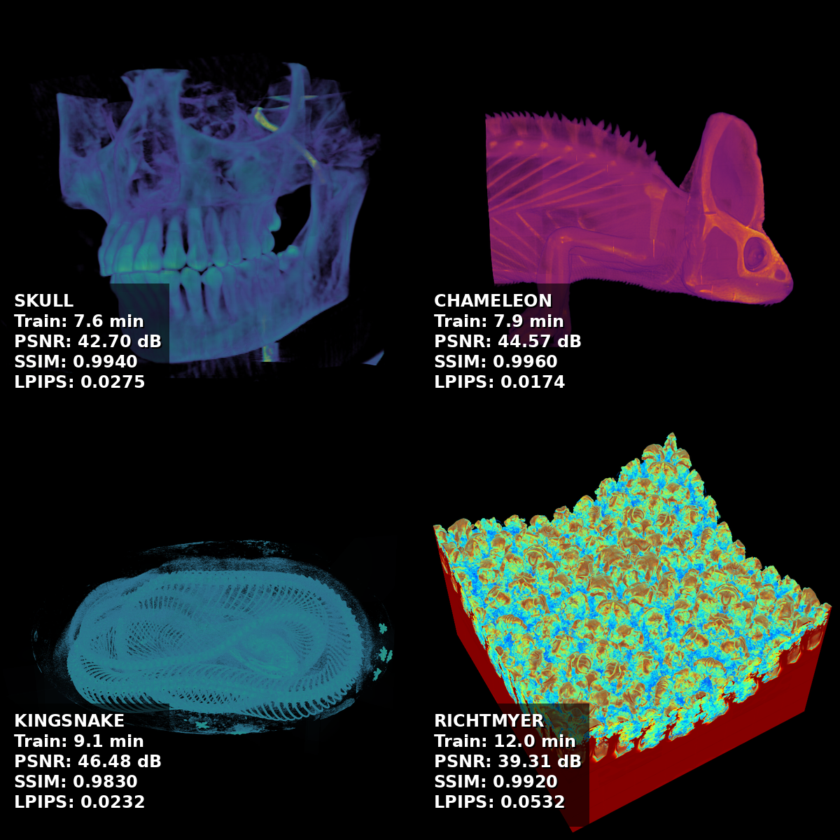
Independent standard-GS optimizers can each densify freely. This gives them enough capacity for high-frequency structures, but their aggregate primitive count grows with the number of domains. The MCMC variant divides the primitive count of a monolithic GS baseline among all subdomains, keeping the global budget nearly constant and reducing both training time and storage.
| Dataset at 256 GPUs | GS PSNR | GS time | MCMC PSNR | MCMC time | MCMC storage reduction |
|---|---|---|---|---|---|
| Skull | 42.70 dB | 454.66 s | 35.32 dB | 265.31 s | 60.07x |
| Kingsnake | 46.48 dB | 547.35 s | 29.51 dB | 318.76 s | 112.5x |
| Chameleon | 44.57 dB | 476.43 s | 41.23 dB | 290.57 s | 161.3x |
| RMI | 39.31 dB | 718.45 s | 22.15 dB | 263.37 s | 71.6x |
Storage reduction compares aggregate standard-GS and bounded-MCMC model footprints at 256 domains. Training time is the total time-to-solution reported by the evaluation.
The memory bound is not free. MCMC works well when a downloadable model size is a hard constraint, but a monolithic primitive budget can starve complex local optimizers. On turbulent RMI data, bounded MCMC falls to roughly 22 dB at 256 domains; unrestricted GS is the appropriate choice when fidelity is the priority.
Temporal Fine-Tuning
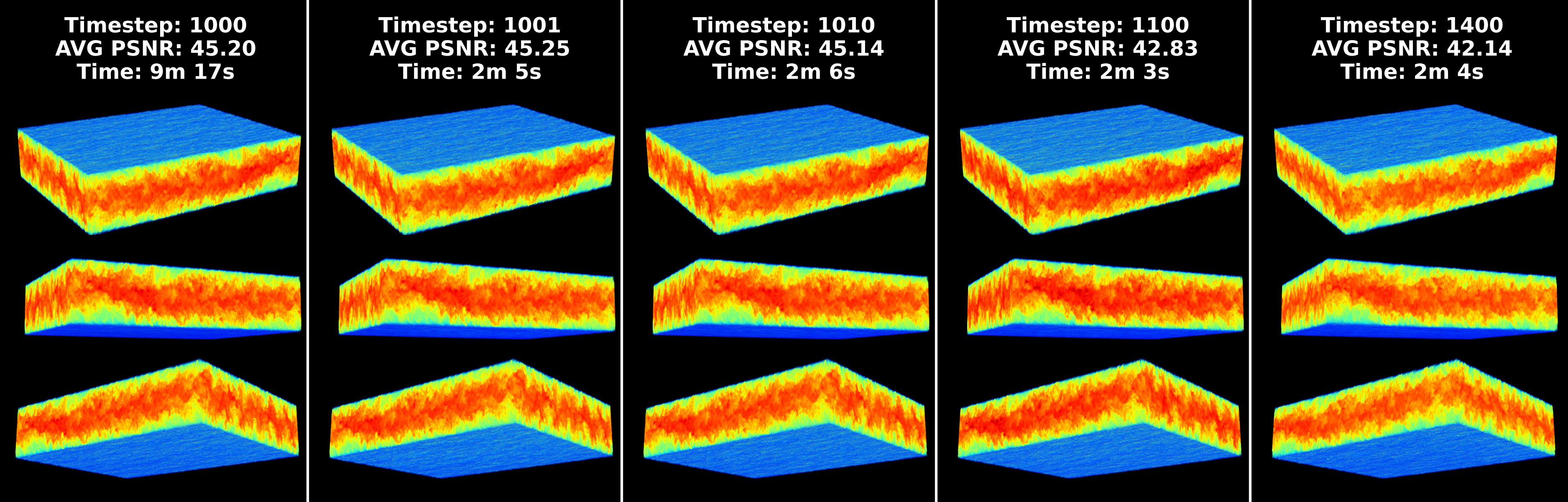
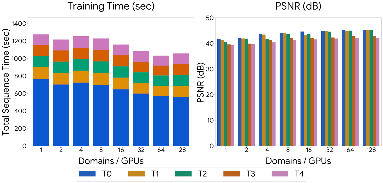
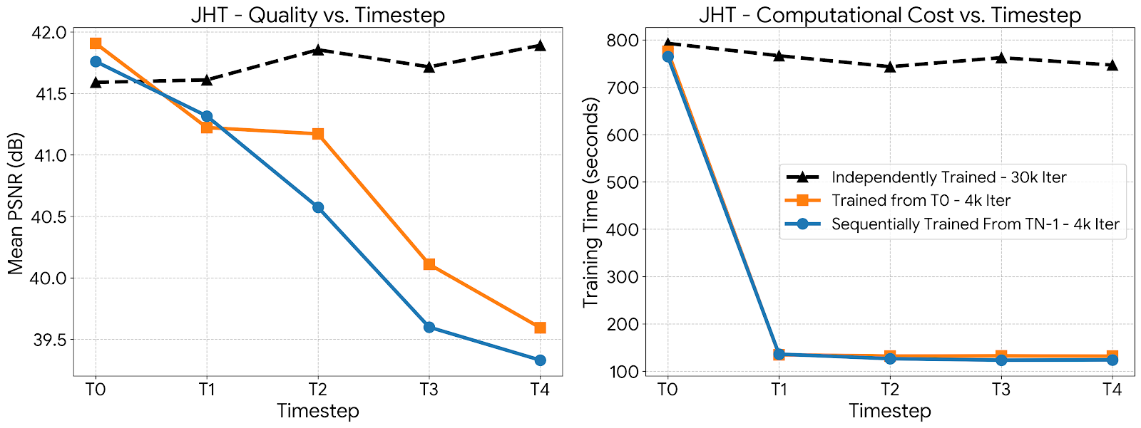
The first simulation step is trained from voxel initialization for 30,000 iterations. Each later step starts from the optimized positions, covariances, spherical harmonics, and colors of the preceding model and fine-tunes for 4,000 iterations. At 128 GPUs, the baseline takes 557 seconds and subsequent steps take about 124-127 seconds.
| 128-GPU timestep | Initialization | Iterations | PSNR | Training time |
|---|---|---|---|---|
| 1000 | Voxel samples | 30,000 | 45.20 dB | 557.06 s |
| 1001 | Previous step | 4,000 | 45.25 dB | 125.87 s |
| 1010 | Previous step | 4,000 | 45.14 dB | 126.60 s |
| 1100 | Previous step | 4,000 | 42.83 dB | 123.36 s |
| 1400 | Previous step | 4,000 | 42.14 dB | 124.19 s |
Quality declines as the physical interval between test frames grows. Fine-tuning every step sequentially and fine-tuning each step directly from the original baseline show similar degradation, indicating that physical change, rather than compounding optimization drift, is the dominant cause.
Practical Configuration
Limitations
- Aggregate model growth: unrestricted standard GS can produce a distributed model larger than the source volume. MCMC bounds storage but can underfit high-frequency data.
- Visual-complexity sensitivity: small, low-detail partitions may lack enough local features to constrain optimization, reducing PSNR at very high domain counts.
- Tail latency: overall training finishes when the slowest partition converges. A future asynchronous task queue could improve utilization.
- Distributed rendering: local models render at 237-450 FPS at single-domain scale, but IceT compositing limits the 256-domain result to roughly 9-11 FPS.
- No direct concatenation: fragment clipping depends on per-domain bounds, so local models cannot be joined into one artifact without a global boundary-aware fine-tuning pass.
BibTeX
@article{sewell2026scalable,
  author = {Sewell, Andres and Han, Mengjiao and Wu, Qi and Petruzza, Steve},
  title = {Scalable Training and Rendering of 3D Gaussians for Large-Scale Scientific Data},
  journal = {Proceedings of the ACM on Computer Graphics and Interactive Techniques},
  year = {2026},
  volume = {9},
  number = {4},
  articleno = {55},
  numpages = {25},
  publisher = {Association for Computing Machinery},
  doi = {10.1145/3820022},
  url = {https://doi.org/10.1145/3820022}
}